
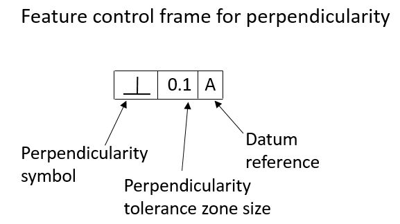
Perpendicularity
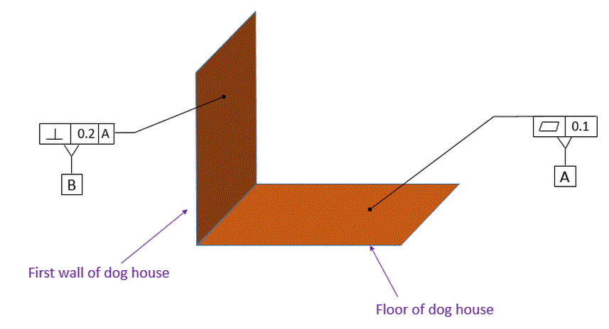
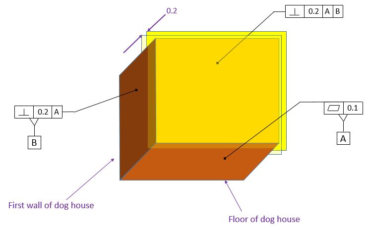
If we want to build a dog house, we will probably start out with a nice flat floor. We can specify how flat we want the floor by using a Flatness Tolerance. Then we will start building our walls. Our floor is horizontal, and we want our wall to be vertical. So we want our wall to be perpendicular to the floor.

We have labeled our floor datum [A]. Now we need to specify that our wall must be perpendicular to the floor. The feature control frame for the perpendicularity tolerance is shown below:
We apply the perpendicularity control to the wall as shown below. Our perpendicularity control specifies that perpendicularity must be held within 0.2 relative to datum [A].
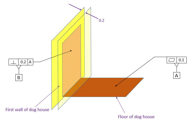
The figure below shows the tolerance zone for our perpendicularity control. The tolerance zone is two parallel planes that are 0.2 apart and that are exactly perpendicular to datum [A].
Because the entire surface must fall within this tolerance zone, the flatness of the surface is controlled as well as the angle.
Because the entire surface must fall within this tolerance zone, the flatness of the surface is controlled as well as the angle.
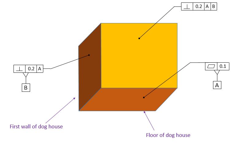
Next we will want to add the rear wall. We will want the rear wall to be perpendicular to both the floor and the first wall. So we apply a perpendicularity control to the rear wall. The perpendicularity control specifies that the rear wall must be perpendicular to both datums [A] and [B].
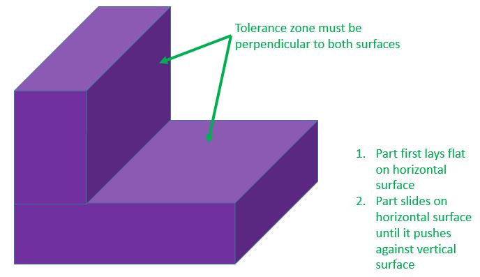
The figure below shows the tolerance zone for the back wall. The tolerance zone is perpendicular to both datum [A] and datum [B].
In order to understand datums [A] and [B], it's helpful to consider the gage in the figure below. While the bottom and side of the dog house are designated as datum features, it's the gage that represents the datums. The datums are perfect planes. Datum [A] is tangent to datum feature [A]. Datum [B] is perfectly perpendicular to datum [A]. Datum feature [B] will likely only have two points of contact with the surface of the gage that simulates datum [B]. So While datums [A] and [B] are perfectly perpendicular to each other, the bottom and side wall of the dog house are not.
In order to gage the rear wall of the dog house, the floor is first laid flat on the gage. Then the dog house is slid until the side wall contacts the vertical wall of the gage in at least two points. The tolerance zone for the back wall is perpendicular to the bottom and side surfaces of the gage, not the floor and side wall of the dog house.
In order to gage the rear wall of the dog house, the floor is first laid flat on the gage. Then the dog house is slid until the side wall contacts the vertical wall of the gage in at least two points. The tolerance zone for the back wall is perpendicular to the bottom and side surfaces of the gage, not the floor and side wall of the dog house.
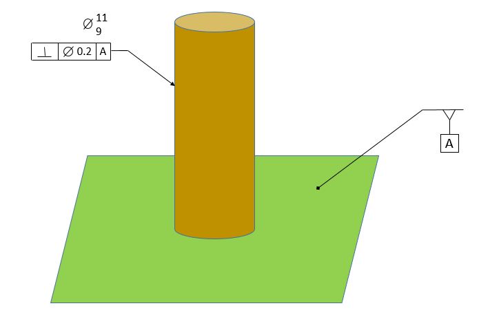
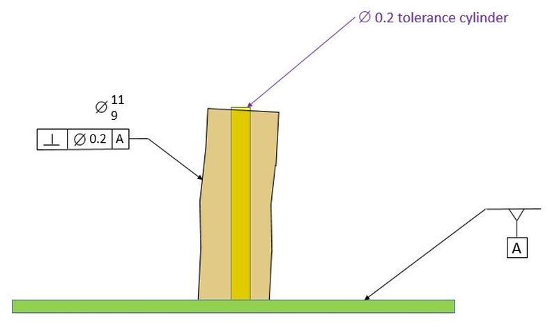
Now we will apply perpendicularity to a fence post for a dog pen. We will consider the ground to be flat and horizontal. We want our post to be perpendicular to the ground. We specify the ground to be datum [A]. We specify that our post must be perpendicular to datum [A] within 0.2
Note that the feature control frame now has a diameter symbol in the box with the tolerance. The diameter symbol indicates that the tolerance zone is a cylinder.
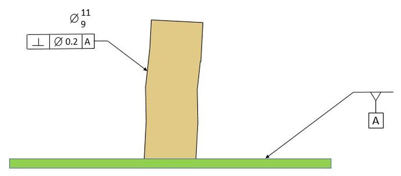
The figure below shows the ground and our post in a true view. In the real world, the post will not be perfectly straight and it will not be perfectly perpendicular to the ground.
The requirement for our perpendicularity control is that the axis of the post must fall within a tolerance cylinder 0.2 diameter. The tolerance cylinder is perfectly perpendicular to the datum.
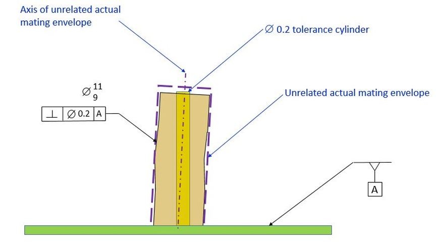
Note that in this case we talk about the axis of the post falling within the tolerance cylinder and later we will look at a boundary that the post occupies instead of looking at the axis. The reason we look at the axis in this case is that the perpendicularity is called out Regardless of Feature Size (RFS). When we specify something at RFS, we look at the axis. Later we will use the MMC modifier. When we do that, we will look at boundaries. The next issue to deal with is the fact that we are supposed to look at an axis of something that is not straight. So we must define the axis of a crooked post.
Note that in this case we talk about the axis of the post falling within the tolerance cylinder and later we will look at a boundary that the post occupies instead of looking at the axis. The reason we look at the axis in this case is that the perpendicularity is called out Regardless of Feature Size (RFS). When we specify something at RFS, we look at the axis. Later we will use the MMC modifier. When we do that, we will look at boundaries. The next issue to deal with is the fact that we are supposed to look at an axis of something that is not straight. So we must define the axis of a crooked post.
We define the axis of the post as being the axis of the unrelated actual mating envelope of the post. As we recall, the unrelated actual mating envelope is the smallest perfect cylinder that will fit over the post. It is not related to any datums, so it is not necessarily perpendicular to datum [A]. The axis of the perfect cylinder is what must fit inside the 0.2 diameter tolerance cylinder for the perpendicularity control.
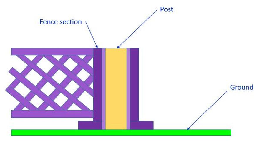
Now if we want to fit a section of fence over our post, we need to make sure that the fence section will always fit over the post. We see below how this system will work. The post protrudes from the ground. The fence section has a hole that fits over the post. The hole in the fence section must fit over the post while the base of the fence section sits flat on the ground. In order to make sure that the fence section will always fit over the post while the base of the fence section sits flat on the ground, we must look at the Virtual Condition (VC) of the post and of the hole. As long as the VC of the hole is bigger than the VC of the post, our fence section will always fit over the post properly.
To introduce the concept of Virtual Condition, consider the post. Note that now we have included the MMC modifier in the feature control frame. When we use the MMC modifier, we talk about a Virtual Condition (VC). The Virtual Condition is a fixed size boundary that is exactly perpendicular to datum [A]. The size of the Virtual Condition is always a combination of the MMC size and the geometric tolerance. In this case, since the post is an external feature of size, the Virtual Condition size is the MMC size plus the perpendicularity tolerance.
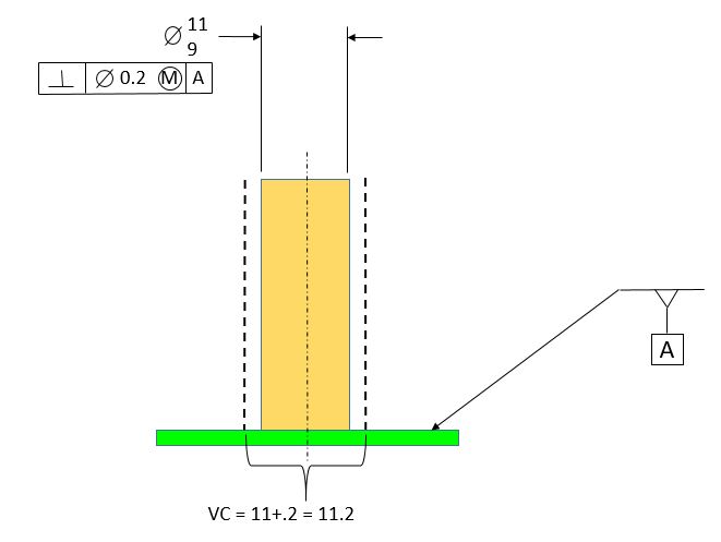
In order to meet the part requirements, the post must meet the size requirements, it must meet the Rule #1 requirement for straightness, and it must be sufficiently perpendicular to datum [A] that it will not fall outside the Virtual Condition boundary.
Note from the animation below that when the post is at its largest allowable size, it can have just a little bit of perpendicularity error without violating the Virtual Condition boundary. As the post gets smaller, but still within its size requirement, it can have more perpendicularity error and still not violate the Virtual Condition boundary. This extra perpendicularity error that is allowed because of the size of the part is called Bonus Tolerance. Bonus tolerance is the extra perpendicularity tolerance we are allowed as a result of the part being smaller than its MMC size. Therefore the amount of bonus tolerance allowed is equal to the MMC size minus the actual part size.
One may ask what is the maximum bonus tolerance allowed by the drawing. Since the maximum bonus tolerance would be allowed when the part is at its LMC size, then the maximum possible bonus tolerance allowed by the drawing is equal to the MMC size minus the LMC size.
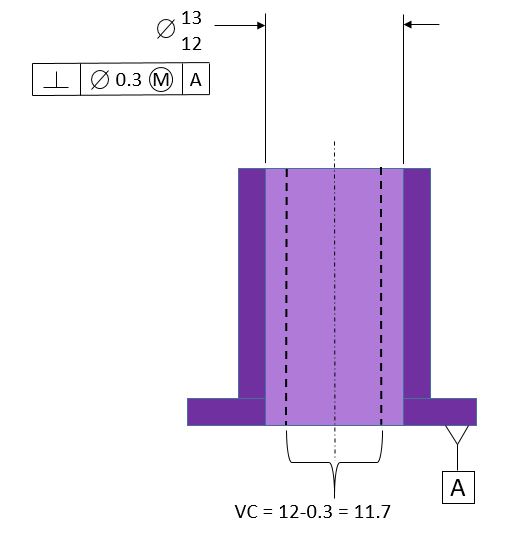
Now we will look at the part of the fence section that slides over the post. Once again we use the MMC modifier, and there is a virtual condition. The virtual condition is a fixed boundary that is exactly perpendicular to datum [A]. Since this is an internal feature of size, the size of the virtual condition boundary is the MMC size of 12 minus the perpendicularity tolerance of 0.3 which makes 11.7
When the hole is at its MMC size of 12, it can have 0.3 perpendicularity error without violating its virtual condition boundary. As the hole gets larger within its size limit, it can have additional perpendicularity error and still not violate the virtual condition boundary. The additional perpendicularity error allowed because of the size being bigger than the MMC size is called bonus tolerance. The amount of bonuse tolerance allowed is equal to the size of the hole in a given part minus its MMC size. The maximum bonus tolerance that a hole is allowed to have is equal to its LMC size minus its MMC size.
Now we know that the fence section will always fit over the post. They are both constrained by boundaries that are perpendicular to datum [A]. The post will never go outside of its 11.2 boundary and the fence section will never violate its 11.7 boundary.